Rate of penetration optimization using machine learning technique

Introduction

A key challenge confronting the oil industry, particularly in drilling, is the high cost of drilling, which has garnered significant focus in recent decades. Several factors influence drilling costs, with the most significant being the well's drilling time, which can substantially raise expenses. Reducing drilling time is a primary objective for drilling engineers. In essence, one of the key goals of optimizing drilling operations is to decrease the overall time required. Two approaches have been suggested to achieve this goal: selecting the optimal drilling parameters (such as choosing the appropriate drill-bit and drilling fluid) and performing real-time analysis to fine-tune operational factors like rotary speed and weight on bit during drilling [1, p. 1-25]. Various approaches were presented for the optimal bit selection program. The traditional method for selecting a drilling bit relies on historical data, including cost per foot (CPF), specific energy (SE), bit wear, offset-well bit performance, and geological details [2, p. 1225-1229]. Most of these methods use Rate of Penetration (ROP) as one of its inputs; therefore, ROP prediction became a valuable means for Bit Selection optimization to reduce drilling time, thus costs. The rate of penetration (ROP) is the primary factor influencing drilling duration. Therefore, the accuracy of the ROP model is essential. Several factors influence the rate of drilling, such as the properties of drilling mud, the characteristics of the formation, the speed of rotation, and the features of the bit [3]. Certain factors are beyond control, like the characteristics of the formation, while others can be controllable, including the Weight on Bit (WOB), drillstring rotation speed (RPM), bit type and size, pump flow rate, and drilling mud properties. The impact of various factors on the (ROP) can be analyzed separately, including parameters such as weight on bit (WOB), revolutions per minute (RPM), and rock strength [1, p. 1-25]. A study analyzing various mathematical models of ROP discovered that the majority of them incorporate factors such as the bit diameter, rotation, and weight on bit, which are either exponentially or linearly adjusted by constants as inputs. The model suggested by Bourgoyne and Young, nevertheless, remains the most widely recognized. Certain parameters they utilize are not always readily accessible, making their model suitable primarily when an extensive amount of well data is available.

Data overview and methodology

From three wells in a Middle East field, a comprehensive dataset is collected and represented by (13575 data points), comprising historical drilling data containing diverse drilling parameters including rotary speed, weight on bit, mud density, etc., along with the corresponding ROP values. For this study, 12 drilling parameter have been selected as the most effective parameters on ROP. Figure 1 shows the heatmap of all drilling parameters of these three wells.

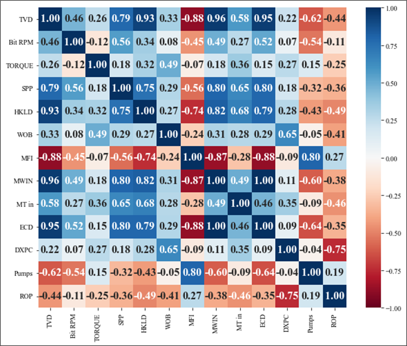
Fig. 1. Heatmap chart for 13,575 data points for the three wells

From this heatmap the most important parameters that were considered to develop the SVM ROP Model as inputs are listed below:

• True Vertical Depth (TVD) (m).
• Bit Rotary Speed (RPM) (1/min).
• Torque (T) (Ft*Lb).
• Hook Load (HKLD) (Ton).
• Mud Weight (sg).
• Stand Pipe Pressure (psi).
• Pump Flow Rate (SPM).
• Weight On Bit (WOB) (Ton).
• Mud Temperature In (℉).
• Mud Flow In (gpm).
• Equivalent Circulation Depth (ECD) (sg).
• D Exponent.

Data cleaning

It is important to minimize the errors of collected data that might was produced during data capturing or editing prior to storing, to maximize the usefulness and significance of the data. Failure to perform routine data cleaning can result in accumulated errors, which may hinder efficiency and create future challenges [4]. There many methods to complete the data cleansing process, statistical method was implemented in this research by examining the data utilizing the values of range, standard deviation, mean, etc. where the aim was to reduce the standard deviation for the selected parameters of the collected data, while maintaining the median and main values are close to the original values as much as possible. Data pre-processing and cleaning are needed before feeding any ROP model. The quality of the data is directly linked to the outcomes produced by any model. The last stage of this process involves identifying and eliminating outliers, which are data points that deviate significantly from the majority of the dataset [5, p. 181-185]. Such data are often anticipated to emerge within extensive experimental datasets. Such data can influence the precision and dependability of models [6, p. 694-701]. Therefore, obtaining this data is crucial for the advancement of models [7, p. 88-100]. At first, when they are easily recognizable, the process can be carried out manually. However, after this stage, more advanced techniques become essential. In this research, Interquartile Range (IQR) method was evaluated. Figure 2 show the boxplot of some input data that has been used to determine the outliers, mean and median of these data.

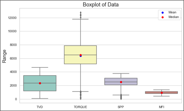
Fig. 2. Box plot of dataset

This study utilizes the leverage approach to identify outliers as well. The discrepancy between the predicted values and the corresponding experimental data was calculated using this method.

Data pre-processing (normalization)

Prior to feeding the input-output data into the training phase of any model, all datasets were scaled to a range of [-1, 1] using Equation (1), where X is the input parameter, is the normalized value of input parameter, and and are the maximum and minimum values of input parameters, respectively. In fact, the scaling of data within these ranges [-1, 1] is an important task to be performed in order to prevent computational issues and comply with algorithmic criteria [8, p. 339-354].

, (1)

The outliers also must be removed as a data cleansing process, the results of this process, which is called Data Cleansing, are summed up in table 1. The processed data, deemed valid and exhibiting a normal distribution, were considered reliable, therefore, used to build and train ROP Model. Once the data screening, filtering, and outlier removal processes were finished, the dataset used to develop the SVM ROP Model consisted of 11,336 records.

Table 1

Parameters cleansing statistical data

Support vector machine (SVM)

In this research, we developed SVM model with a Radial Basis Function (RBF) kernel to forecast the Rate of Penetration (ROP) in drilling operations. The model's performance was assessed by testing different combinations of the cost parameter (C) and gamma (γ) [9]. The objective was to determine the optimal combination of these parameters that minimizes the Root Average Squared Error (RASE) and reduces the R² value, indicating a better fit and generalization capability of the model.

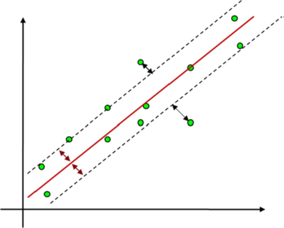
Fig. 3. Concept of ε-insensitivity in the linear data analysis [10, p. 515-535]

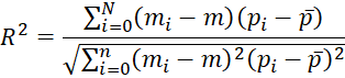
Performance measures

To check how well does the developed model truly represent the set of data, the forecasting capacity of the model were determined by using two performance criteria: the mean square error (MSE) and the determination coefficient . The and MSE values can be calculated utilizing Eqs. (2) and (3), respectively.

, (2)

, (3)

Where 𝑝̅ and 𝑚̅ are the standard deviation and mean of the recorded values, respectively; pi and mi are the recorded and simulated values at step i, respectively; n is the number of samples in the database [11].

Results and discussion

Detailed comparison between SVM ROP Model output with real-life measured data were performed, supported with graphical and statistical representation of the created ROP Model outputs against real life data. Differences between ROP Model output and real-life measured data was calculated to measure the errors which is a measure of quality, precision, and uncertainty of the developed Model. This error analysis is used to determine the accuracy of SVM model for ROP prediction, and to examine its suitability to simulates the physical behavior.

Support vector machine (SVM) ROP model

The model's performance was assessed through different combinations of the cost parameter (C) and gamma (γ), as shown in table (2). The SVM model was developed and validated using a comprehensive dataset, with the (C) and (γ) values systematically varied ten times producing ten models to determine their impact on the model’s performance.

Table 2

SVM ROP model selection after building 10 models

Upon evaluating the performance metrics, it was evident that model number 7 with Cost (C): 4.72 and Gamma (γ): 0.24. This combination yielded the highest R² value of approximately 0.8945 and the lowest RASE values across the test, validation, and training datasets. Specifically, the Training RASE was 1.97, the Validation RASE was 1.95, and the Test RASE was 1.84. These findings suggest that the model is highly accurate and generalizes well, making it the optimal choice for predicting ROP.

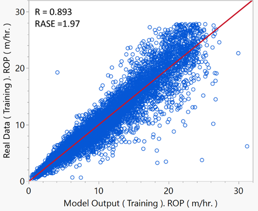
Fig. 4. Cross-Plot of SVM ROP Model Outputs vs. Real Data (Training Data Set)

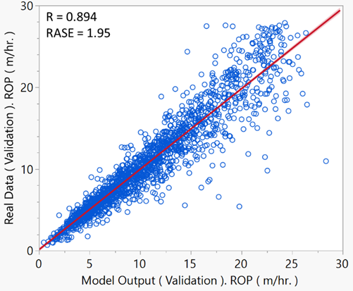
Fig. 5. Cross-Plot of SVM ROP Model Outputs vs. Real Data (Validation Data Set)

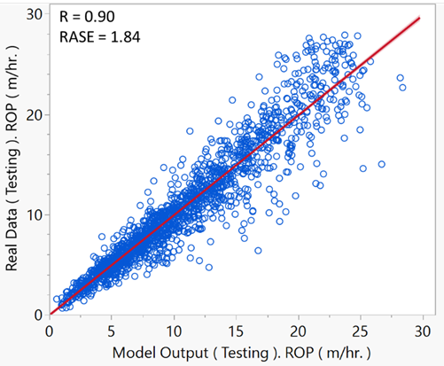
Fig. 6. Cross-Plot of SVM ROP Model Outputs vs. Real Data (Testing Data Set)

Evaluating the residuals (the difference between predicted and actual ROP) serves as a valuable method for identifying shortcomings in the ROP Model. From figure 7, it is obvious that the mean value of residual error in testing data sets is almost zero, with a standard deviation of residuals around + / -2, which means that the predicted value has a relatively low tolerance of error.

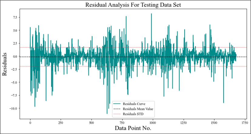
Fig. 7. Residual analyses for testing data set

Conclusions

1. SVM was successfully utilized to develop models for forecasting ROP in a Middle East field.
2. The SVM ROP Model demonstrated a good correlation coefficient (0.893 to 0.90) and RMSE (1.84 to 1.97).
3. Sensitivity analysis revealed that parameters such as "mud flow in" and "pump rate" positively impact ROP, whereas other factors have a negative effect. Among the input variables, the D exponent (DXPC) has the greatest influence on ROP.