Artificial intelligence-based optimization of drilling parameters for enhanced rate of penetration in heterogeneous formations

Overview

Drilling engineering involves the planning, design, and implementation of drilling operations to extract natural resources from the earth's subsurface. It is a complex and challenging task that requires significant expertise and knowledge of geological, mechanical, and operational factors.

A critical challenge in drilling engineering is the reliance on human judgment under dynamic and high-risk downhole conditions. Efforts to reduce operational expenditures often result in suboptimal decision-making, thereby escalating project costs.

Integrating AI into drilling workflows enhances operational precision, minimizes safety incidents, and promotes efficient resource allocation.

The implementation of artificial intelligence (AI) within various scope in oil and gas has been growing rapidly worldwide in recent years. AI technologies are revolutionizing the industry by increasing efficiency, reducing costs, and improving safety.

The implementation of AI in oil and gas is already being used by many companies worldwide. For example:

1. SOCAR (Azerbaijan):

• Name: Methane AI.
• Focus: Methane monitoring.
• Overview: integrates satellite, drone, and ground sensor data to monitor and reduce emissions across operations. The platform uses OGMP recommended formulas to quantify non measured sources using equipment specific standard parameters and build in AI engine can extrapolate measurements from a limited number of sources to the whole infrastructure.

2. SLB:

• Name: Lumi™, Neuro™, OptiSite™
• Focus: AI platforms, autonomous systems, data analytics
• Key Initiatives: Lumi™: AI-powered platform for subsurface insight and decision support (source); Neuro™: Autonomous geosteering system guiding drill bits in real time; OptiSite™: Production optimization using AI and digital twins.

3. Shell:

• Name: Shell Cognitive Bar
• Focus: AI for monitoring, predictive analytics, energy transition
• Key Initiatives: AI system that predicts equipment failures and anomalies; Use of AI and ML to optimize refining and trading; Partnerships with startups to deploy AI in carbon tracking and optimization.

4. Equinor:

• Focus: Offshore operations, digital twins, predictive analytics
• Key Initiatives: Partnered with SLB to achieve autonomous drilling; Uses AI for real-time reservoir modeling, drilling optimization, and emissions tracking.

Introduction to Neural Networks application in Drilling

Artificial Neural Networks (ANNs) are computational models inspired by the structure and functioning of the human brain. They consist of interconnected processing units (neurons) capable of learning complex relationships from data. Neural networks are particularly powerful in tasks such as classification, approximation, regression, signal processing, pattern recognition, and system identification.

Neural networks are implemented as predictive and diagnostic tools for drilling operations. Using offset well data, feedforward neural networks are trained to forecast key drilling parameters and predict potential downhole complexities such as stuck pipe, lost circulation, or kicks. Neural Network Toolbox (NNTool) serves as a primary platform for prototyping, training, and validating these models. The networks are optimized using algorithms like Levenberg-Marquardt and evaluated through accuracy metrics and generalization performance on unseen test datasets.

This implementation enables more informed decision-making in real-time drilling operations and supports the development of intelligent drilling advisory systems based on data-driven insights.

Examples of using neural network technology for digital signal processing include: filtering, parameter estimation, detection, system identification, pattern recognition, signal reconstruction, time series analysis, and compression. These types of processing are applicable to a variety of signals: audio, video, speech, images, message transmission, geophysical, radar, medical measurements (ECGs, EEGs, pulse), and others.

Signal processing using NN technologies is carried out either with memoryless NNs or NNs with memory. In both cases, the key component is the memoryless NN. This is due to the fact that with certain activation (transfer) functions, a NN acts as a universal approximator. This means that within a given range of input variables, the NN can reproduce (model) any continuous function of those variables with a specified accuracy.

Once the NN structure is chosen, its parameters must be set. As for the parameter values, they are usually determined in the process of solving an optimization problem. This procedure is called training NN theory.

The NNTool GUI allows users to select NN structures from a wide range and offers many training algorithms for each network type.

The following topics related to working with NNTool are covered:

• data preparation;
• creation of a neural network;
• training the network;
• network simulation.

Basic Structure:

• Input layer: Where your raw data (e.g., WOB, ROP, torque) from offset wells enters.
• Hidden layers: Layers where computations are performed. The network adjusts the weights of the connections to reduce prediction errors.
• Output layer: Produces the final result – such as drilling parameters.

For drilling, ANNs can incorporate multiple inputs such as:

• Weight on Bit (WOB).
• ECD.
• Drilling torque (kN*m).
• Pressure (atm).
• Rotary Speed (RPM).
• Mud Flow Rate (l/s).

The goal is to map these inputs to the output variable (ROP) using supervised learning.

At their core, neural networks consist of layers of interconnected neurons. These neurons take inputs (such as well depth, rate of penetration, or mud weight), apply a mathematical transformation, and pass the result to the next layer. Through this structure, neural networks can learn nonlinear relationships that are difficult to capture using traditional statistical methods.

The goal is to map these inputs to the output variables (i.e. ROP) using supervised learning.

Method and materials

For validation purposes, drilling parameters were gathered from a designated field in the Caspian Sea, utilizing data from three previously drilled wells to train the system and predict operational parameters for a fourth well.

1. Data Collection

Data were collected from a specific drilling field, including real-time operational parameters and corresponding ROP measurements.

2. Input of Initial Data

Start by collecting a dataset that includes:

Dependent variable (Y): Rate of Penetration (ROP)

Independent variables (X)

X₁ = MW

X₂ = Flow Rate (l/s)

X₃ = Pressure (atm)

X₄ = ECD

X₅ = Drilling torque

X₆ = RPM

X₇ = WOB

These values are entered into a data analysis tool

3. Build a Regression Model

Apply multiple linear regression to establish a mathematical relationship between the ROP and the two independent variables.

Y = β₀ + β₁X₁ + β₂X₂ + ⋯ + βₙXₙ

Where:

Y is the dependent variable (the outcome to predict).

β₀ is the intercept term (the value of Y when all X variables are zero).

β₁, β₂, ..., βₙ are the coefficients for each independent variable, representing the effect of each X on Y.

X₁, X₂, ..., Xₙ are the independent variables (predictors).

4. Forecasting Using the Regression Model

Using the equation above, we calculate predicted values of mechanical speed for given combinations of depth and pressure.

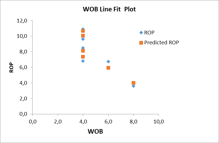
Fig. 1

5. Summary

We combined regression modeling with exponential smoothing to:

1. Predict future values.
2. Smooth the forecasted output for better operational decisions.

6. Network Design and Training

Several network architectures were evaluated using Neural Network Toolbox.

A typical configuration used:

• 6 input neurons (representing WOB, RPM, etc.)
• 1 hidden layer with 10 neurons.
• 1 output neuron (ROP).

The Levenberg–Marquardt backpropagation algorithm was used for training due to its efficiency in function approximation tasks.

7. Results

Table

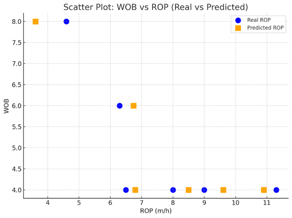
Fig. 2

The ANN model exhibited robust predictive performance, characterized by minimal error rates and high correlation coefficients between forecasted and actual ROP values. The average percentage error is less than 10%

Visual comparisons showed a close match between predicted and real ROP trends.

The results validate the potential of ANN models to provide accurate and real-time predictions of ROP. Compared to empirical methods, ANNs adapt better to nonlinear patterns and field-specific conditions. However, model performance depends heavily on the quality and diversity of the training dataset. Further improvement can be achieved by incorporating more geological and real-time downhole data.

Conclusion

ANNs offer a powerful tool for ROP prediction in drilling operations. ANN models can efficiently model the complex relationships between drilling parameters and ROP, contributing to improved drilling optimization and cost-efficiency. Future work should focus on hybrid models combining ANNs with physics-based approaches and expanding training datasets across multiple fields.