Determination of the coordinates of unmanned aerial vehicles

Russia's global navigation system GLONASS (Global Navigation Satellite System) has been operating since 1982 and was initially used exclusively for the defense interests of the USSR. Since 1987, it has served international cooperation for civil consumption, shipping.

The GLONASS system consists of three subsystems (sections):

1. Space;
2. Surface;
3. Consumption subsystem.

The space segment consists of 24 satellites oriented in three orbital planes (with 8 satellites each). The satellites orbit in a circular orbit at an altitude of 19,100 km, with a rotation period of 11 hours and 15 minutes and an inclination of 64.8°.

This position of the satellites allows the consumer to observe the satellite day and night anywhere in the world.

The terrestrial subsystem provides the architecture of the GLONASS interstellar satellites described above and consists of:

• Control center of system;
• GLONASS signal synchronization system;
• Surface measurement points network (SMP). Provides measurement of orbit parameters of SMPGLONASS satellites and sends them to the ship for information service and control signals;
• A network of quantum-optical stations (NQO) designed for the calibration of SMPs.

The consumer subsystem includes a large number of consumers (military, civilian) with suitable navigation devices.

The American GPS (Global Positioning System) system has similar subsystems and the same operating principles.

The GPS space segment also consists of 24 satellites and are grouped into 6 planes with 4 satellites each. The satellites move in the orbital circle at an altitude of 20180 km with a rotation period of 12 hours and an inclination of 55°. This can be illustrated as follows:

The elements of the GPS surface segment are as described above. However, there is no SME in GPS.

GPS tracking systems are available not only in the United States but also in many parts of the world.

As mentioned above, the working principle of GLONASS and GPS is the same. Therefore, we will cover the following principles together and focus on the individual characteristics of the systems if necessary.

 Global satellite navigation systems, according to their principles, belong to the passive type mid-orbital rangefinder-Doppler system. The passive organization of the system means that users do not send signals to observation satellites, allowing them to serve an unlimited number of consumers of navigation information. In such systems, navigation determinants (coordinate calculations) are primarily created on the basis of measured distances to the satellite. In addition, the nature of satellite signals can be used to calculate both the velocity and the user coordinate of the Doppler displacement frequency of the frequency carrier.

Usually, the signal emitted by GPS's i-th satellite systems has an individually measured code (belonging only to a particular satellite). Thus, according to this code clock, the propagation (propagation) of the signal allows, according to the receiver's clock, to determine the time interval  between the satellite moments (instances) and the moment of receiving the signal of the user antenna.

In the GLONASS system, signals are divided according to frequency between satellites and codes in the GPS system. For this reason, GLONASS satellites emit signals at different frequencies. In the GPS system, the frequency is accurately recorded. Therefore, the GLONASS system uses an entire close range system (1602, 5625-1615, 5000 MHs and 1246, 4375-1256, 9375MHs).

Information processing algorithms. The process of determining location, speed and direction according to the data provided by multi-channel GLONASS / GPS receivers actually combines two different subjects. So, this is a matter called code measurements (pseudo distances and pseudo speeds) and is determined on the basis of the receiver's navigation transmission. The second task is to determine the angular position and angular velocity of UA in one or another coordinate system. The solution is solved by processing phase measurements. It should be noted that it is impossible to solve the second problem without solving the first problem.

The variety of uncontrolled (stochastic, indeterminate, fuzzy) factors and their mutually complex nature provide a constructive approach to the problem of analyzing the UA’s position, velocity and direction on the basis of GLONASS / GPS technology.

Note that the following mathematical models and algorithms need to be developed to model the process of determining the position, speed, and direction of the UA:

• GLONASS/GPS zodiac model;
• GLONASS/GPS observation model of satellites;
• UA center of gravity and angular motion patterns;
• GLONASS/GPS model of navigation sendings;
• Model of the UA's antennas system;
• Algorithm for determining the speed and position of UA;
• UA direction determination algorithm.

Note in advance that all listed models and algorithms must be designed taking into account the following uncontrollable factors:

• GLONASS / GPS system IPS (information pole star) (NIPS) navigation ephemeris errors, due to the detection of the NIPS sky logger by the ground navigation kits and occurring during the management of this satellite system.
• Systematic and random errors in measuring pseudo-distance and pseudo-speeds. These errors are called ionosphere and troposphere delays and occur as a result of servicing the receiver's clock and internal noise.
• Systematic and random errors in measuring the phase differences of frequency carriers. These errors are called multiple beam effects and occur as a result of servicing the receiver's clock and internal noise.
• Systematic and random system placement errors. These errors occur as a result of incomplete knowledge of the initial conditions of the motion.

The following can be used as an algorithm to process information received from the receiving device.:

• Bayesov's iterative algorithm (replacement of Kalman filter);
• Least squares method in complete selection. Determining the position, velocity and direction of the UA using multichannel GLONASS / GPS receivers can be solved if it is equipped with a UA antenna system and with at least 4 antennas placed symmetrically on the symmetrical horizontal plane of the UA.

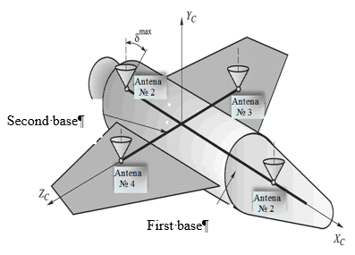
Pic. 1. Antenna’s allocation schema

The problem of determining the component vector of the coordinates and velocity of the UA is solved on the basis of the so-called distance and pseudo-velocity entering the receiver input from the NIPS, which is visible at a given moment of the GLONASS / GPS system. In this case, as a rule, depending on the model of the receiver, either the least squares method (LSM) or Bayesov's recursive prediction algorithm using the UA's built-in motion model is used to solve the problem.

We will then assume that the UA's orientation problem has been completely resolved on the basis of a selected LSM. Therefore, each NIPS created on the basis of the two main bases of the antenna system is used as a measure of the phase differences of the frequency carriers. Such an assumption allows to solve this problem without using a mathematical model of the angular motion of UA or a highly simplified form of this model.

As mentioned above, the analysis of the accuracy of the solution of a similar problem, taking into account various uncontrolled factors, is carried out by simulating the operation of the UA navigation system based on the GLONASS / GPS system multi-channel receiver. In this case, the built-in implementation of the algorithm is taken into account for a wide variety of measurement errors. Finally, the accuracy feature can be obtained by statistical analysis of the UA direction navigation process based on the Monte Carlo method.

         Now let's move on to the explanation of the mathematical model of the GOLNASS / GPS system used in the NIGU movement. It was mentioned above that two types of NIGU motion models of the GOLNASS / GPS system were used in simulation modeling. The first type of model is used to model the "real" motion of the NIGU. The second type of model can be thought of as a "built-in" model with integrated onboard navigation system and part of the mathematical software of maneuver UA.

The simulated mathematical model of NIGU allows the ephemeris of these CAs to be formed with the necessary accuracy. Therefore, given the following deviation explanations:

• Non-centralization of Earth's gravitational field, including up to 8 harmonic orders and degrees;
• The gravitational force of the Sun and Moon;
• Aerodynamic resistance of the atmosphere;
• Sunlight pressure.

A high precision Dorman-Prince method can be introduced to integrate the system of differential motion equations of NIPS. Because the method can automatically check local errors and the length of the integration step. Subsequent use of the resulting ephemeris can be accomplished, for example, by Chebeshev's polynomial approximation.

The built-in model of the NIPS movement can be realized using a very simple motion model considering the following.:

• Decentralization of Earth's gravitational field including accuracy and degree of up to 2 harmonic rows;
• The gravitational force of the Sun and Moon.

In this case, the standard Runge-Kutta method (2/6 rule) with a fixed integration step can be introduced for the integration of NIPS's system of differential equations of motion.

It is important to use the "coarse" ephemeris of the "real" NIQU as the initial conditions for integration for the "on-board" model of NIPS movement. Thus, they are obtained for about half an hour on the basis of the imitation model. The "roughness" is performed on the basis of the law of normal distribution of ephemeris errors characterized by the following properties of the covariance matrix:

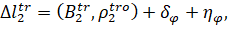
The IPS ephemeris error of the NIPS is determined by the following values of the orbital normals and along the orbit and along the radius of the orbit:

  (1)

The built-in multi-channel navigation receiver uses two types of models as well as a mathematical model of the movement of the grouped UA:

1. A "real" motion model used to shape the actual trajectory of the UA, including the UA's direction, position, and velocity;
2. Built-in model using integrated navigation and tracking systems built into the RPT.

The "real" motion model includes the maximum exact differential equation system of spatial motion related to the geographic coordinate system of the UA.

GLONASS / GPS technology, used in the creation of the mathematical software of the embedded integration system, has a special place not only in determining the position and speed of the UA, but also in defining the direction of the coordinate system and all possible relationships between them.

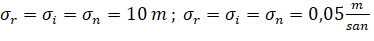
As a result of the analysis, it was revealed that the minimum set must contain the following coordinate systems in order for the card to be applied (pic. 2):

Pic. 2

• 2000.0 inertial coordinate system (IF-2000). The beginning of IF 2000 calculation is located in the center of gravity of the Earth.

Main flatness – 0ⁿ 00^m 00^s middle Ecuador (J 2000,0 time) shows.

X_İF  axis points to the middle of the spring equinox. ZIF axis 1900-1905 years, according to an international agreement, the Earth was oriented on the axis of rotation. YIF axis completes the coordinate system to the right.

• Location-related coordinate system (LRC).

The starting point of the LRC is located at the center of mass of the Earth. The ZLRC axis is directed to the Earth's axis of rotation according to the International Conventional Principles of 1900-1905. The XLRC axis crosses the Greenwich ladder with respect to the corresponding International Conventional Start. YLRCoxu completes the coordinate system on the right.

• Orbital coordinate system (OF).

The calculation start of OF is located at the center of mass of UA. The XOF axis is directed to the radius vector of UA called the R axis. The ZOF axis is oriented in the direction of the momentum vector of UA's motion. This axis is called the N axis. YOF axis completes the coordinate system to the right (called the L-axis). Related coordinate system (BF).

The computational origin of BF is located at the center of mass UA. BF axises (X0, Y0, Z0) form the symmetry axes of UA.

The coordinates of the antennas are given in the corresponding coordinate system. It is necessary to determine the visible NIPS and calculate the distance vector and recalculate the coordinates and components of the velocity vector of each antenna in the inertial coordinate system for derivative distances. Let us show the relationships that describe the transitions between the coordinate systems used for this.

Let us include the matrix operators for the rotation of each axis about any angle "a":

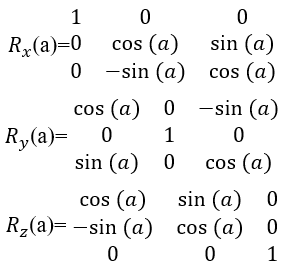
Then the transition matrix from the inertial coordinate system to the  Greenwich coordinate system can be written as:

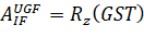 ,      (2)

GST – Greenwich Standard Time.

The transition matrix from the inertial coordinate system to the  orbital coordinate system is written as follows.:

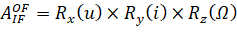,   (3)

Here, i, u – indicates the time, slope and latitude argument of the nodes UA, respectively.

The transition matrix from the orbital coordinate system to the  – linked coordinate system is written as follows.

When the antenna's coordinates are in the – linked coordinate system, R_S-UA are the coordinates of the center of mass.

In an inertial coordinate system, the velocity vector of the antenna can be written as.

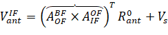,     (6)

When  is the coordinates of antennas in the corresponding coordinate system, VS – UA is the velocity vector of the center of mass.

The exact position vector of the antenna in the inertial coordinate system is as follows:

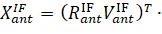  (7)

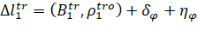
Now let's move on to the explanation of mathematical measurement models that determine the direction of the solution of the navigation problem in the given order. This can be done similarly to the formation of an action model. Here, too, two types of models can be used: the "real" measurement model and the "embedded" model, which are used for direct information processing.

Two measurement channel models are used in simulation modeling.

The "real" measurements model, in other words the imitation model, is realized by the following relationships.

Measurement of length.

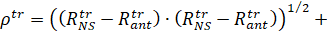
        (8)

Where,

P^tr – UA’s distance between antennas and NIPS is "Real" value.

 – NIPS is “ Real ” radius vector.

 is the "real" radius vector of antennas in an inertial coordinate system.

 displays systematic errors between NIPS timescale and receiver;

ℵ_p – indicates systematic errors caused by the ionosphere capacitance of the signal;

ηp – indicates random additional errors caused by internal noise of the receiver.

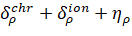
Derivative distances are measured as follows.

    (9)

Where,  UA’s distance between antennas and NIPS is "Real" value;

 is “real” vector of NIPS’s speed;

 is the "real" radius vector of antennas in an inertial coordinate system;

 is a single vector in the direction of the "true" distance between the UA antenna and the NIPS.;

systematic errors of measuring the scanning distance.

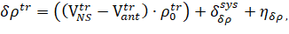
Measuring the phase difference.

The figure below explains the schematic diagram of measuring the phase difference of the frequency carriers of the NIPS signal. Thus, NIPS is placed in the field of view of both antennas of UA satellite navigation devices. Here m-k is the integer number of wavelengths of the frequency difference of the NIPS signal so that the base ϑ of the first and second antennas is taken. (ϑ is an indefinite integer parameter);

∆φ – is NIPS the measured phase difference of the signal;

 is a single vector of the line of sight from object to NIPS.

These measurements determine the values of the protrusions of the antenna base to the nearest centimeter in the visibility direction of the visible NIPS, so the final result is to determine the orientation of the object in phase.

The receiver directly measures the missing values of the projections. The exact values of the projections are determined algorithmically.

The following equivalent linear quantity can be taken as the measured value of the phase difference of the main bases of the antenna system:

,    (10)

Where, ,  – are the "True" values of the phase difference of the first and second bases;

 is the "Real" vector of the first and second bases calculated in the inertial coordinate system.;

1 and 3 "True" are true vectors in the direction of the distance between antennas and NIPS;

δφ systemic errors associated with multiple effects of signal reflection.

The systematic error associated with excessive radiation of the signals received by the GLONASS / GPS receiver has a correlation coefficient (δφ ) that depends on the angle difference over the local horizon of the NIPS, and measurements are performed sequentially as follows:

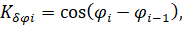 (11)

Where, φ1 is the spread angle of the NIPS from which the measurement is made, 

φi-1  – is the spread angle of the NIPS from which previous measurements were made,

φ  – random additional errors caused by internal noise from the receiver.

On-board models used in information processing are realized in the following ways.

Distance measurement:

,    (12)

Where,

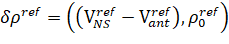
Pref  is the support value of the distance between the UA antenna and the NIPS;

 – NIPS is the support radius vector;

 is the support radius vector of antennas in inertial coordinate systems.

Measurement of derivative distances.

,      (13)

Where,

 – Derivative distances between UA antennas and NIPS are support values;

 – NIPS is the support vector of speed;

 download reference vectors of the velocities of UA antennas in the inertial coordinate system;

 – support between UA antennas and NIPS is a single vector in the direction of distances.

The following equivalent linear quantities can be considered as measured values of the phase difference n of the main bases of the antenna systems B1 and B2:

      (14)

,    (15)

Where, ,  is the difference between the supporting phases of the first and second bases.

 the first and second bases are support vectors;

 – 1 and 3 are unit vectors in the direction of support distances between antennas and NIPS.

Depending on the type of receiver used to process login information, two types of algorithms can be used.:

1. Bayesov's iteration algorithm based on the age of the Colman filter modification.
2. The traditional least squares method that works in the selection of exact measurements.

In the first case, it is recommended to use a modification of the Kalman filter called "scalar" modification, since the main feature is that the components of the measurement vector are sequentially processed and the use of matrix transformation is avoided. It is more convenient to present the functionalization process of the "scalar" modification of the Kalman filter in the form of the following scheme: J=1....,N_S  where N_S - is the number of sessions that determine the coordinates and components of the velocity vector. P_j covariance estimation matrix

  (16)

Where Ф_j,j-1  is a basic matrix of system navigation assignments in a session.

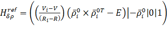
The prognostic vector of the UA state is the integration of differential equations of motion of UA's center of mass with respect to time .

Calculation of support distance up to i-th, NIPS, observation matrix of the distance is as follows:

,    (17)

Where,

 – is i-th single vector in the direction of distance to NIPS.

∆X computing the state vector change:

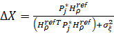    (18)

Calculation of Pi pre-covariance matrix:

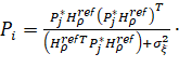   (19)

Computing the state vector X_j:

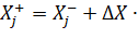  (20)

calculation of derivative distances in the direction, observation matrices for  velocities:

,   (21)

Here, Ri, Vi is the i-th NIPS position and velocity in the inertial coordinate system. R, V is the position and velocity of UA in the inertial coordinate system.

Then, similar to the previous ones, the change of state vector ∆X, matrix P and new formula Xj are calculated according to the above formula.

The second type of algorithm – the fully selection least squares method – is the traditional method of processing orbit measurements; Here, as a set of measurements, a set of distances and derivative distances are taken in the direction up to each visible NIPS. Observation matrices for each measurement are calculated using the above formulas.

The multi-channel receiver of the GLONASS / GPS system can also be used to determine the direction of the UA and the least squares method with full selection. It is important to note the following features of the given algorithm:

• The set of phase difference values of the two main antenna bases before each visible NIPS is used as the measurement sequence;
• Observation matrices for each measurement are determined by the numerical complexity of the relationships that measure and evaluate the parameters.

1. Веремеенко К. К., Тихонов В. Л., Кудрявцев В.М., Ходаков А. В. Интегрированный навигационно-посадочный комплекс / Сб. трудов Международной конференции «Планирование глобальной радионавигации». Т. 2. С. 7-10.
2. Веремеенко К. К., Музылев И. Г., Зайцев А. С. Навигационно-посадочный комплекс на основе спутниковых навигационных систем / Тезисы докладов «Аэрокосмические приборные технологии». Национальный симпозиум с между народным участием. Москва, 28 мая - 1 июня 1999. С. 11-12.
3. Веремеенко К. К., Денисов В. И., Карпов А. С. Исследование характеристик инерциально-спутниковых навигационных систем / Матери докладов Всероссийской молодежной НТК «Приборостроение в аэрокосмической технике». Арзамас, 1999. С. 97-99.
4. Веремеенко К. К. Интегрированные инерциально-спутниковые навигационные системы: проблемы и перспективы развития / Доклад на Международных научных чтениях, посвященных памяти И. Сикорского. – Москва, май 2001.
5. ВеремеенкоК. К., Тихонов В.А. Навигационно-посадочный комплекс на основе спутниковой радионавигационной системы // Радиотехника. 1996. № 1, выпуск 8.
6. Интегрированные инерциально-спутниковые навигационные системы / Под ред. Пешехонова. – С.-Петербург, 2001. – 235 с.
7. Веремеенко К. К. Оценка возможностей идентификации погрешностей вектора выходных параметров БИНС и инструментальных погрешностей ее измерительных элементов путем комплексирования со спутниковой системой навигации в процессе полета // Гироскопия и навигация. 1996. № 1B. С. 74-75.
8. Веремеенко К. К., Красов А. И., Стулов А. В., Шестаков И.Н. Авиационные спутниковые приемники-индикаторы фирмы Trimble. – М.: МАИ, 1998. – 107 с.
9. Глобальная навигационная спутниковая система ГЛОНАСС. Интерфейсный контрольный документ (редакция четвертая). КНИЦ МО РФ, 1998.
10. Вавилова Н. Б., Голован А. А., Парусников Н. А., Трубников С. А. Математические модели и алгоритмы обработки измерений спутниковой навигационной системы GPS. Стандартный режим. – М.: МГУ, 2001.
11. Шебшаевич В. С, Дмитриев П. П., Иванцевич Н. В. и др. Сетевые спутниковые радионавигационные системы. – М.: Радио и связь, 1993. 1998. Interface Control Document GPS 200C, Revision IRN-2Q0C-Q02, ARINC Research Corporation, 1997.
12. Малышев В. В., Красильщиков М.Н., Бобронников В. Т. и др. Спутниковые системы мониторинга. – М.: МАИ, 2000.
13. Bartenev V.A., Krasilshchikov M.N., Malyshev V. V. and oth. Russia's global navigation satellite system, ANSER Ohio, USA, 1994.
14. Андреев В. Д. Теория инерциальной навигации, ч.1. Автономные системы. – М.: Наука, 1966.
15. Помыкаев И. И., Селезнев В. П., Дмитроченко Л. А. Навигационные приборы и системы. – М.: Машиностроние, 1983.
16. Бромберг П. В. Теория инерциальных систем навигации. – М.: Наука, 1979.
17. Ривкин С. С, Ивановский Р. И., Костров А. В. Статистическая оптимизация навигационных систем. – Л.: Судостроение, 1976.