Tax income prediction using Markov Decision Process

Introduction

Decisions are a fundamental feature of society and we make quite a lot of them every day. These choices not only result in a reward, but they also have an influence on future decisions. We may not accomplish a high overall performance if we neglect the effect today's decisions have on future decisions, as well as current and future advantages. Markov decision processes provides a mathematical framework that takes these characteristics of decision making into account [1].

Traditional decision analysis is widely used to handle complicated problems in a variety of disciplines. The level of complexity makes it necessary to use more sophisticated modeling approaches. The standard decision tree was the most often used approach for evaluating decision analysis issues in the past [3]. But standard decision trees were not efficient in modeling complicated situations as they have plenty of serious limitations, especially when results or events occur (or may repeat) from time-to-time. As a result, conventional decision trees are frequently replaced with Markov process–based techniques for modeling recurring states and future occurrences.

The decision-making model is as follows: A decision maker analyzes the system state at a specific point in time. The decision maker makes a choice based on available data. This action has two possible outcomes. First, the decider gets rewarded instantly, and the system evolves to a new state at the next point in time based on a probability distribution established by the action being taken [6]. The decision maker is currently in the same predicament. However, the decision maker may be in a new system state this time, presenting him with fresh actions. Main components of the model are below

• epochs - are set of decision times. We name the points of time in which decisions are made the decision epochs. 
• state space - a set of system states.
• set of possible actions to make. At every decision epoch it can be assumed that the decision maker is in some kind of state. At certain decision epoch, the decision maker examines he is in some state, and he chooses an action, that he is allowed to make in state.
• the costs or rewards that depend on actions or states
• transition probabilities that depend on states or actions described in state space.

Markov decision processes are one of the stochastic sequential decision processes. In general, the Markov decision process is all about memoryless processes. Main idea is that the future state of some process is dependent only on its present case. Any of the past cases were not taken into account while choosing the next state.

Stochastic processes have now become a popular tool for mathematicians, physicists, and engineers, with applications ranging from stock price modeling to rational option pricing theory to differential geometry. Markov decision processes are effective analytical tools that have found widespread usage in a variety of industrial and manufacturing applications such as transportation, finance, and inventory control. Markov decision processes expand standard Markov models by including the sequential decision process into the model and allowing for numerous decisions across various time periods [4]. A Markov model is a stochastic model used to represent pseudo-randomly changing systems in probability theory. It is thought that future states are determined only by the current state and not by previous occurrences. In general, this assumption allows the model to be used for reasoning and computation that would otherwise be impossible. As a result, it is desired for a given model to display the Markov property in the disciplines of predictive modeling and probabilistic forecasting. Markov decision processes (MDP) can be categorized into finite-horizon and infinite-horizon MDP’s according to the time interval in which decisions are made. Finite-horizon and infinite-horizon MDP’s both have various analytic properties and that’s why different solution algorithms. When transaction probabilities and reward functions are stationary infinite-horizon MDP’s are preferred over finite-horizon type MDP. Because in those cases optimum solution of finite-horizon MDP with growing planning horizon approaches to equivalent infinite-horizon MDP and to solve and calibrate infinite-horizon MDP’s is easier than it is in finite-horizon MDP [5]. However, in some cases stationary expectation is not logical for example when transition probability represents disease outcome which is increasing over the time and death probability is depends on some factors like age of the person [2].

Markov model methodology

Transition probability matrices are estimated for 2016-2020 for sub-items of tax revenues. The estimator of the transition probabilities is the relative frequency of the actual transitions from phase i to phase j, i.e. the observed transitions have to be divided by the sum of the transitions to all other phases.

In this paper, 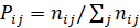 where i, j = A, B, C, D, E and n_ij is the number of observed transitions from i to j and  is the sum of observed transitions from i to j.

Frequency distribution of the realization rate intervals must be mutually exclusive (non-overlapping) and class width must be equal for each interval. Transition probabilities from  to , i, j = 0,1,2,…,n , can be constructed as the following matrix

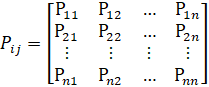
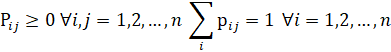
Since P_ij are constant and independent of time (time homogeneous), matrix P_ij=P is called a stochastic matrix. P_ij probabilities must satisfy the following conditions:

Given that data at time n is in state X₀ and that the data will be in one of states X₀ ∈{0,1,2,...} at time n+1, then the data at time n+2 can be predicted. Given initial probability P(X₀=i) = p_i for every i, the required probability is matrix multiplication . Equivalently, next year’s probability distribution matrix can be predicted by

Initial probability matrices for four Markov models are 1xj row matrices. Stationary prediction matrices Q_n+1 have a limiting matrix Q, which can be written as .

Best of Four Markov Models

For every year of the sample and for every Markov model, mean square error (mse) is calculated by 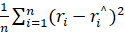 where i is the number of states 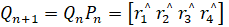is predicted realization rate at time n+1 and 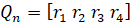is observed realization rate at time n. The least mse gives the best Markov model.

Variations between observed and expected frequencies can be tested by constructing a contingency table of frequency distribution of transitions between the states at 0,05 significance level with a degree of freedom.

To validate Markov model, for every year, the value of the χ² statistic is computed based on the null hypothesis, H₀: model is valid. At 0,05 level of significance and with the degrees of freedom, the χ² critical value and χ² test value are estimated. The null hypothesis is not rejected whenever χ² test value is less than the critical value. Test values are calculated by 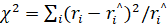 where i is the number of categories, r_i and  are the actual and estimated values, respectively.

Income tax realization rates from smallest to largest are classified as E,D,C,B, A in model 1, D, C, B, A in model 2, C, B, A in model 3 and B, A in model 4. For years between 2016 and 2020 table 2 shows that realization rates are over 100% in three categories of model 1, in two categories of model 2, in two categories of model 3.

Table 1

For the years 2016-2020, the realization rates of income tax, classes and transitions for four Markov models are shown in Table 2 (numbers are given in 000 AZN format).

Table 2

Prediction of cost table shows possible coefficient

Table 3

Optimum value of income tax amount can be calculated by recent years collected tax amount multtiplied by prediction of cost values from the table.

=0.1·6432906.7+ 0.2·6553378.8+0.7·7548941.2+0·7864370.1+0·6501948.2 =7238225

=0.08·6432906.7+0·6553378.8+0.08·7548941.2+0.4·7864370.1+0.44·6501948.2 =7125153

=0·6432906.7+ 0.5·6553378.8+0.25·7548941.2+0.25·7864370.1+0 ·6501948.2 =7130017

=0.12·6432906.7+0.13·6553378.8+0.5·7548941.2+0·7864370.1+0.25·6501948.2 =7023846

=0.25·6432906.7+ 0.7·6553378.8+0 ·7548941.2+0·7864370.1+0.05·6501948.2 =6520689

=0.3·6432906.7+0.2·6553378.8+0.2·7548941.2+0.3·7864370.1+0·6501948.2=7109647.04

=0.2·6432906.7+0·6553378.8+0.7·7548941.2+0·7864370.1+0.1·6501948.2=7221035

=0·6432906.7+0·6553378.8+0.3·7548941.2+0.4·7864370.1+0.3·6501948.2=7361014.86

=0·6432906.7+0.1·6553378.8+0.25·7548941.2+0.6·7864370.1+0.75·6501948.2=12137656

=0.1·6432906.7+0.6·6553378.8+0·7548941.2+0·7864370.1+0.3·6501948.2=6525902.41

=0·6432906.7+0.2·6553378.8+0.7·7548941.2+0·7864370.1+0.1·6501948.2=7245129.42

=0.2·6432906.7+0·6553378.8+0.4·7548941.2+0.4·7864370.1+0·6501948.2=7451905.86

=0·6432906.7+0.6·6553378.8+0.25·7548941.2+0.75·7864370.1+0.3·6501948.2=13668124

=0.35·6432906.7+0.65·6553378.8+0·7548941.2+0·7864370.1+0·6501948.2=6511213.57

=0.25·6432906.7+0.7·6553378.8+0.7·7548941.2+0·7864370.1+0.05·6501948.2=11804948

=0.1·6432906.7+0.3·6553378.8+0.3·7548941.2+0·7864370.1+0.3·6501948.2=6824571.13

=0.5·6432906.7+0·6553378.8+0.2·7548941.2+0.2·7864370.1+0.1·6501948.2=6949310.43

=0·6432906.7+0.5·6553378.8+0.25·7548941.2+0.25·7864370.1+0·6501948.2=7130017.23

=0.13·6432906.7+0.25·6553378.8+0.5·7548941.2+0·7864370.1+0.12·6501948.2=7029326

=0.25·6432906.7+0.7·6553378.8+0·7548941.2+0·7864370.1+0.05·6501948.2=6520689.25

Table 4

Table of results shows all the calculation results and maximum possible values

Result of the calculation show that maximum value is P1 = 7451905.86.

Conclusion

Markov decision process can be used to find optimum values of given problem with high accuracy. In this article we used this method to predict tax realization rates of next years.