Speech synthesis with preset speaker emotions using Tacotron architecture

Introduction

Speech synthesis directly represents the generation of a speech signal based on printed text by restoring the shape of the speech signal from its parameters. It should provide generation of speech with natural sounding, preserving to a proper extent the parameters of the speaker's voice.

Speech synthesis systems started their way back in the XX century, but received a serious boost in development due to the active introduction of deep learning and today they are capable of producing results almost identical to human speech. This has allowed them to find application in many fields, from audio books to customer self-service systems in various spheres or generation of voice for use in media products.

However, there are no universal solutions that can produce equally good results when generating speech with certain characteristics: speech is not always natural and lively or emotional. One of the problems leading to this is that the speech synthesis system becomes too accustomed to the parameters inherent in the training sample – from the voice characteristics of a particular speaker to the range of his emotions. For this reason, such systems require certain presets that can adjust the sound of synthesised speech to the task at hand.

As one of them, it can be considered speaker's emotion preset during speech synthesis, which will allow generating speech within a specific emotion, rather than obtaining a generalised less emotional speaker's sound based on his audio data.

Methods

The implemented subsystem is based on the existing open-source neural network Tacotron 2.

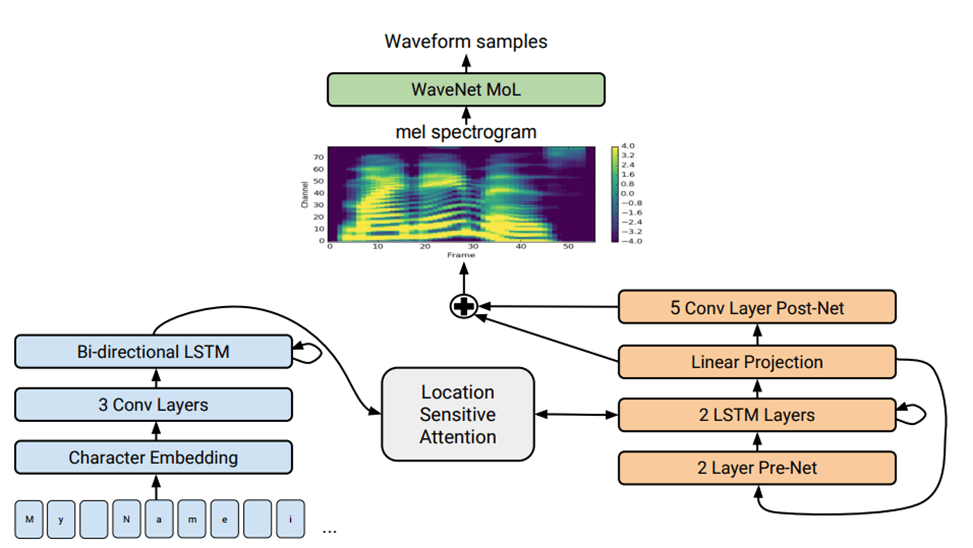
Tacotron is a neural network which is using deep recurrent networks for speech synthesis, consisting of two main modules: a module for converting mel-spectrograms into a wave signal and a module for generating a mel-spectrogram based on a textual description. Its architecture is presented lower (pic. 1).

Pic. 1. Tacotron 2 architecture

Its second module consists of several layers, including a textual symbol embedding layer representing the input text as vectors, several LSTM (Long short-term memory) layers, which are more advanced implementations of standard recurrent networks for context transfer, and several convolutional layers for speech feature generation and transfer [1].

Before proceeding further with this architecture, it is important to review its main elements mentioned earlier:

• convolutional networks (CNN);
• long short-term memory networks (LSTM) - a more advanced form of recurrent neural networks architecture (RNN);
• character embedding layer for obtaining a vector representation of the input characters.

1. Convolutional networks. They are predominantly used for image processing, but can also be applied to audio data processing. For example, a spectrogram of an audio track can be represented as an image.

The convolution layers perform a convolution operation using a set of filters applied to the input image and allow the extraction of local features. After the convolution operation, a ReLU (Rectified Linear Unit) activation function is usually used.

A convolutional neural network has the following structure:

1. The convolutional layers.
2. Pooling layers.
3. Fully connected layers.

The layer is called a convolution layer because it provides the convolution computation. It is described by the following formula:

, (1)

where:

f[n₁, n₂] – the brightness values of the image pixels;

g[x – n₁, y – n₂] – filter weights.

2. Recurrent Networks. While convolutional networks have been applied mainly to images, recurrent networks are actively used in natural language processing (NLP). These are networks that contain inverse connections and allow information to be stored.

The idea behind a recurrent network is that information is used sequentially and all data is processed in a context-aware manner. This is useful when it is required to predict the next word in a sentence based on the previous one. Thus, recurrent networks are an excellent option for processing sequential data, which can include both text and audio.

The structure of the recurrent network is as follows:

1. Input vector x at some step t.
2. The hidden state h_t at step t, which is updated while processing the input data sequence.
3. Output y at step t.

The RNN performs the processing of sequential input vectors x based on the recurrence formula:

, (2)

where:

h_t – a new state;

f_w – some function with parameter w;

h_{t - 1} – old state;

x_t – the input vector at some step t.

Any recurrent neural network takes the form of a chain of recurrent neural network modules. In a conventional RNN, the structure of one such module is very simple, for example, it can be a single layer with activation function tanh (hyperbolic tangent). Then the formula can be rewritten as follows:

, (3)

where:

W – weight matrix.

3. LSTM neural networks. LSTM is a kind of recurrent network that solves the vanishing gradient problem inherent in the conventional RNN.

The structure of LSTM also resembles a chain, but the modules look different. Instead of a single layer of the neural network, they contain as many as four, and these layers interact in a special way. LSTM contains structures called gates:

• Input gate i – decides whether to write information to the cell.
• Forget gate f – decides whether to erase the cell.
• Output gate o – decides how much to expand the cell.
• Gate gate g – decides how much information to write to the cell [2].

Formula (3) for LSTM will be transformed into the following form:

, (4)

Two states are computed for LSTM: h_t – cell state and c_t – cell memory state, which is updated proportionally to g and forgotten proportionally to f. They are computed using the following formulas:

, (5)

, (6)

4. Embedding (Embedding) layer – translates the input text into a vector representation. These vectors will be trained in conjunction with the rest of the neural network.

The conversion of words into vectors is done based on the following matrix transformation:

, (7)

where:

W – trained matrix of word vectors of size V*D, V is the number of words in the dictionary, D is the length of the vector representing the word;

x – matrix of size N*T, containing rows consisting of T sequentially presented word numbers, for each word number from x a row (vector) from W is selected, N*T vectors of length D are obtained;

out – output matrix of word vectors in the order of their succession, matrix form (N, T, D).

Results

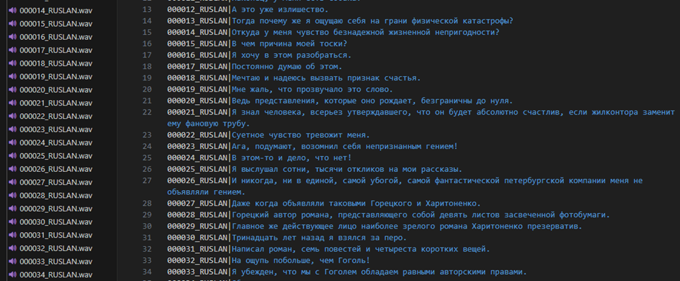
To realize the subsystem of speech synthesis with predefined speaker's emotions on the basis of Tacotron 2, it was decided to install a repository with this neural network, as well as a RUSLAN dataset containing a huge number of speaker's replicas in Russian with text transcriptions to them. Next in the paper could be seen the audio files themselves and their transcriptions (pic. 2).

Pic. 2. Audio files with transcriptions from the dataset

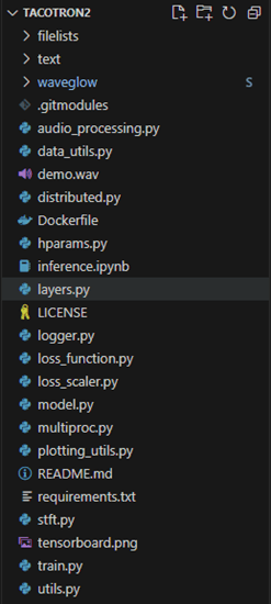
The structure of the Tacotron 2 network is shown further (pic. 3).

Pic. 3. The structure of Tacotron 2 network

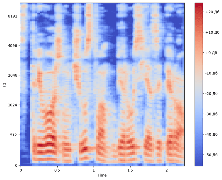
During the training of the model for speech generation, preprocessing of the training audio data was performed: since the Tacotron 2 neural network does not work directly with audio data, but with their Mel-spectrograms [3, p. 143]. Next picture shows the spectrogram of the audio file taken from the sample (pic. 4).

Pic. 4. Mel-spectrogram

Spectrograms for all other recordings of the speaker were obtained in a similar manner and then processed to feed the input of the neural network.

Training was carried out on a small sample of 50 audio tracks, as the goal of this work was not to obtain the highest quality speech, but only to test the implementation of the subsystem of synthesis of emotional speech and understand how it can be improved in the future.

The essence of the implemented subsystem in training the network was to determine which values on the Mel-Spectrogram most of all correlate with the speaker's emotion, which needs to be amplified when reproducing the final result.

The results obtained during network training in terms of speech quality or naturalness do not surpass the standard Tacotron 2 implementation, but they allow to identify the main features of the speaker responsible for his emotions, which in combination with the formation of a dataset marked by emotions will allow to achieve more accurate and qualitative results in the future.

Conclusion

The implemented subsystem based on the Tacotron 2 neural network architecture did not give an increase in the efficiency of speech synthesis by the network, nor did it become an alternative implementation. However, it allowed to understand how a number of resulting parameters can be improved without having to redesign the entire network architecture, but only by working with the speaker's features. It is obvious that the current implementation is not self-sufficient and requires at least modification, and at most – the formation of a specialized dataset for it and the creation of a separate architecture that would give it more flexibility in terms of highlighting the emotions of the speaker.